Physics · ArtemisThermalBase

Every facet of the terrain is treated as the top of its own one-dimensional regolith column. Facets talk to each other only through light: they shadow each other from the Sun and, optionally, warm each other in the infrared. Heat does not flow sideways between columns, which is a good approximation when cells are much wider than the thermal skin depth (a few centimetres for the diurnal wave, under a metre for the annual one).

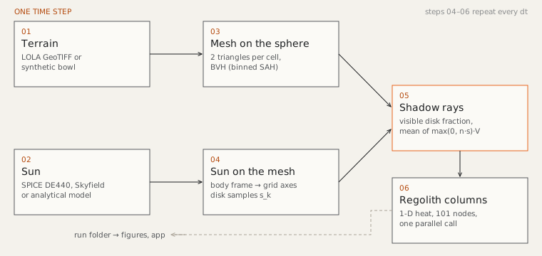
Fig. 1 One time step. Terrain, mesh and BVH are built once; the Sun, the shadows and the conduction step repeat.

At the surface of facet \(i\) the balance is

\[ \underbrace{(1-A_i)\,S(t)\,F_i(t)}_{\text{sunlight}} + \underbrace{Q_{\text{IR},i}(t)}_{\text{terrain}} \;=\; \varepsilon_i\,\sigma\,T_{s,i}^4 \;-\; k\left.\frac{\partial T}{\partial z}\right|_{z=0}, \]

and below it heat diffuses down to a geothermal flux at the bottom. The sections below go through each term.

Terrain and frames

A DEM with \(n_y \times n_x\) points becomes \(2(n_y-1)(n_x-1)\) triangles, two per grid cell, each with its own normal, area and centroid. Before that, every vertex is lowered by the height of the lunar sphere below the tangent plane at the DEM centre,

\[ \Delta z = R - \sqrt{R^2 - x^2 - y^2}, \]

115 m at 20 km. A flat DEM would let distant terrain stand too tall and cast long shadows that do not exist; with the Sun 1.5° above the horizon, 115 m at 20 km is 0.3°.

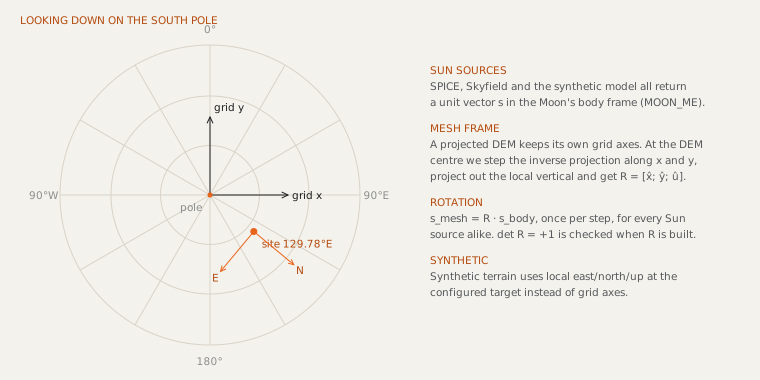
The Sun direction has to arrive in the same frame as the mesh. Real DEMs come in a map projection (polar stereographic for the poles), whose \(x\) and \(y\) axes are not east and north except along one meridian. We take the DEM centre, step the inverse projection by 10 m along \(x\) and along \(y\), convert those points to unit vectors on the sphere, remove the local vertical, and build a right-handed rotation \(\mathbf R = [\hat x;\,\hat y;\,\hat u]\) from the lunar body frame to the mesh. Synthetic terrain uses local east, north and up at the configured site instead. A test checks \(\mathbf R\) against the same construction with the DEM’s own CRS through rasterio.

Top-down view of the south pole with map grid axes, a site at 129.78°E and its local east and north directions — Fig. 2 At the site, the map's grid axes are rotated by about 130° from local east and north. Using one for the other turns every shadow.

Where the Sun is

Three sources, one interface: each returns the unit vector from the Moon to the Sun in the lunar body frame and the Sun’s distance.

SPICE: NAIF DE440 with the lunar principal-axis kernel, in the mean-Earth/polar-axis frame MOON_ME, light-time and stellar aberration corrected. Kernels are pinned by SHA-256. This is the research path.
Skyfield: The Moon-to-Sun vector from a JPL kernel (DE421 by default), rotated into the body frame with the IAU 2015 lunar orientation model, including its thirteen periodic terms. Against SPICE MOON_ME it is within 0.003° between 2025 and 2030. Fine for previews; research mode does not accept it.
Synthetic: The sub-solar point sits at a fixed latitude and travels once around the Moon per synodic month, starting at local noon over the site. Near the pole that keeps the Sun a degree or two above the horizon and moving in azimuth all day, which is what the polar Sun does. It needs no data and is the default.

Irradiance at the Moon is \(S(t) = S_0\,(1\ \text{AU}/d(t))^2\) with \(S_0 = 1361\ \text{W m}^{-2}\) (Kopp & Lean 2011). The synthetic Sun uses \(S_0\).

Shadows and penumbra

The Sun is 0.53° wide, a third of its height above the horizon at the pole. A point Sun would make every shadow edge a step; in reality a facet can see part of the disk. We place \(N\) directions \(\hat s_k\) over the disk on a Fibonacci spiral (equal solid angle each, 16 by default, 64 for research) and cast one shadow ray per direction from just above the facet centroid.

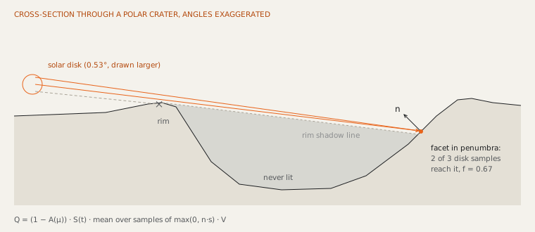
Cross-section of a crater with a low Sun: the near rim casts a shadow line onto the far wall, one of three disk rays is blocked by the rim — Fig. 3 A facet near the shadow edge sees part of the disk. The blocked sample ends at the rim.

Two numbers come out per facet:

\[ f_i = \frac1N\sum_k V_{ik}, \qquad F_i = \frac1N\sum_k \max(0,\,\hat n_i\cdot\hat s_k)\,V_{ik}, \]

where \(V_{ik}\) is 1 if ray \(k\) escapes. \(f_i\) is the visible fraction of the disk, used for maps and statistics. \(F_i\) multiplies the irradiance; it is not \(\cos\theta_i \cdot f_i\), which is biased exactly where it matters, on steep walls and when the disk centre is just below a facet’s horizon.

With point_source_mode a single ray goes to the disk centre and \(F_i\) is \(\cos\theta_i\) or 0. Rays are traced through a bounding-volume hierarchy built with a binned surface-area heuristic (16 bins, at most 4 triangles per leaf) and tested with the Möller–Trumbore algorithm in double precision. Faces turned away from the Sun skip the ray altogether.

Absorbed sunlight

\[ Q_{\text{sun},i} = \bigl(1 - A(\mu_i)\bigr)\,S(t)\,F_i, \qquad \mu_i = \max(0,\hat n_i\cdot\hat s). \]

With Hapke enabled (the default), \(A(\mu)\) is the directional-hemispherical albedo of the Hapke (2012) model with mature highland parameters (\(w = 0.23\), double Henyey–Greenstein \(b = 0.21\), \(c = 0.70\), shadow-hiding opposition \(B_{S0} = 1\), \(h_S = 0.065\)), integrated over the exit hemisphere once into a 2049-point table in \(\mu\). It falls from about 0.06 at normal incidence to near zero at grazing incidence. Without Hapke, \(A\) is the Bond albedo 0.12.

Terrain infrared

Crater walls lit by the Sun at 300 K radiate onto a floor that the Sun never reaches. With view_factors.enabled, every facet shoots cosine-weighted rays into its upper hemisphere (128 by default, 512 for research). The fraction of rays that hit facet \(j\) first estimates the view factor \(F_{ij}\), stored as a sparse matrix. Each step the facet then absorbs

\[ Q_{\text{IR},i} = \varepsilon_i \sum_j F_{ij}\,\varepsilon_j\,\sigma\,T_{s,j}^4 , \]

one bounce of gray thermal emission, using the surface temperatures of the previous step. Reflected infrared and scattered sunlight are not included. Reciprocity \(A_iF_{ij} = A_jF_{ji}\) implies that each facet sends as much power into the terrain as the terrain sends back to it; the run reports the relative mismatch of those totals. It falls like \(1/\sqrt{N_{ ext{rays}}}\): on a test bowl, 0.16 at 128 rays and 0.08 at 512.

Without terrain infrared, a permanently shadowed floor cools until it radiates away only the geothermal flux, about 21 K. We ran the same lunar day over Shackleton twice, with and without this term:

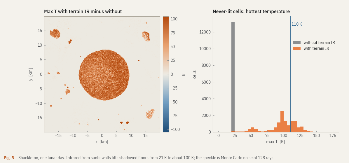
Left: difference in maximum temperature with and without terrain infrared. Right: histogram of the hottest temperature of never-lit cells in both runs — Fig. 4 Terrain infrared changes the answer to the ice question. The area where ice is stable shrinks from 302 to 201 km², and 31 km² become marginal.

Without it the floor never leaves 21 K; with it the median hottest temperature of never-lit cells is 100 K and some reach 150 K. Diviner sees most south-polar cold traps clearly warmer than that (Paige et al. 2010); for crater floors the difference is mostly this term. Turn it on for anything quantitative inside craters.

Emission and roughness

The surface emits \(\varepsilon_i\sigma T_s^4\). Unresolved roughness traps some of the emitted radiation in small cavities, which raises the effective emissivity. We use a simple parameterisation in the spirit of Bandfield et al. (2015):

\[ \varepsilon_{\text{eff}} = \varepsilon_0 + (1-\varepsilon_0)\,K\,\sin\bar\theta,\qquad \bar\theta = \sqrt{\theta_{\text{DEM}}^2 + \theta_{\text{rms}}^2}, \]

with \(\varepsilon_0 = 0.95\), \(K = 0.4\), the facet’s resolved slope \(\theta_{\text{DEM}}\) and a sub-pixel RMS slope \(\theta_{\text{rms}} = 20°\). It moves \(\varepsilon\) by less than 0.02. It is not Bandfield’s full model, which also changes the apparent temperature with viewing angle.

Heat conduction

Below each facet,

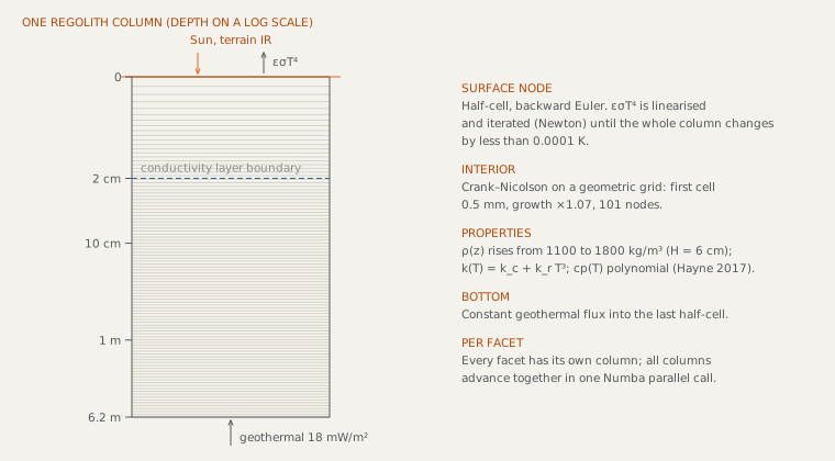
\[ \rho(z)\,c_p(T)\,\frac{\partial T}{\partial t} = \frac{\partial}{\partial z}\left(k(T,z)\,\frac{\partial T}{\partial z}\right), \qquad -k\left.\frac{\partial T}{\partial z}\right|_{z=z_{\max}} = Q_{\text{geo}} . \]

One regolith column: geometric grid on a log depth axis, surface and bottom boundary conditions and the property model — Fig. 5 The column under every facet. Cells start at 0.5 mm and grow by 7 % per layer to 6.2 m.

Grid. 100 layers whose thickness grows geometrically from 0.5 mm by a factor 1.07, reaching 6.2 m: fine enough at the top to resolve the diurnal skin depth, deep enough that the annual wave has died out at the bottom.

Interior nodes use Crank–Nicolson on the non-uniform grid,

\[ C_j\,(T_j^{n+1} - T_j^{n}) = \tfrac12\left[\alpha_j (T_{j-1} - T_j) + \gamma_j (T_{j+1} - T_j)\right]^{n+1} + \tfrac12\left[\cdots\right]^{n}, \]

with \(C_j = \rho_j c_{p,j}/\Delta t\), \(\alpha_j = k_{j-\frac12}/(\Delta z_{j-1}\overline{\Delta z}_j)\), \(\gamma_j = k_{j+\frac12}/(\Delta z_j\overline{\Delta z}_j)\) and interface conductivities taken as harmonic means.

The surface node is a half cell treated with backward Euler. Its radiative loss is stiff: with a 0.5 mm cell, a 300 s step and \(T^4\) in the boundary, Crank–Nicolson can oscillate at sunrise and sunset. The fully implicit step is L-stable and does not. The \(T^4\) term is linearised around the latest iterate,

\[ \varepsilon\sigma T^4 \approx \varepsilon\sigma\left(4\tilde T^3 T - 3\tilde T^4\right), \]

and the tridiagonal system is solved again (Newton iteration, Thomas algorithm) until the largest change anywhere in the column is below \(10^{-4}\) K (at most 20 iterations).

The bottom node is a Crank–Nicolson half cell that receives the geothermal flux, 18 mW m⁻² (Apollo 15 and 17; Langseth et al. 1976). The flux enters the column once, there; it is not added at the surface.

How large a time step is safe is measured in Configuration: 300 s stays within 0.13 K of a 30 s reference over a lunar day.

Regolith properties

Hayne et al. (2017), as used for the Diviner global regolith model:

\[ \rho(z) = \rho_d - (\rho_d - \rho_s)\,e^{-z/H}, \qquad \rho_s = 1100,\ \rho_d = 1800\ \text{kg m}^{-3},\ H = 6\ \text{cm}; \]

\[ k(T,z) = k_c(z) + k_r(z)\,T^3, \]

with \(k_c = 7.4\times10^{-4}\), \(k_r = 2\times10^{-11}\) above 2 cm and \(k_c = 3.4\times10^{-3}\), \(k_r = 10^{-11}\) below (W m⁻¹ K⁻¹ and W m⁻¹ K⁻⁴). The radiative \(T^3\) term makes hot regolith conduct several times better than cold. Heat capacity is the polynomial

\[ c_p(T) = c_0 + c_1 T^{1/2} + c_2 T + c_3 T^2 + c_4 T^3, \]

floored at 8 J kg⁻¹ K⁻¹ so it stays positive near absolute zero.

Starting state and spin-up

A column’s deep temperature remembers months of history, so the starting state matters. By default each column starts isothermal at the temperature that radiates away its day-mean absorbed sunlight,

\[ T_0 = \left(\frac{(1-A)\,\overline{S F} + Q_{\text{geo}}}{\varepsilon\sigma}\right)^{1/4}, \]

with \(\overline{SF}\) from 24 point-source shadow maps spread over one synodic month. This removes most of the start-up transient for the cost of 24 cheap ray-tracing passes. For results, spin-up lunar days are simulated before the recorded period and the change between the last two is reported; research mode requires three.

Ice stability

Water ice exposed to vacuum loses mass at the Hertz–Knudsen rate

\[ E(T) = p_v(T)\sqrt{\frac{m}{2\pi k_B T}}, \]

with the vapour pressure of hexagonal ice from Murphy & Koop (2005), \(\ln p_v = 9.550426 - 5723.265/T + 3.53068\ln T - 0.00728332\,T\) (Pa). At 110 K that is \(4.5\times10^{-15}\) kg m⁻² s⁻¹, a metre of ice in about 6 billion years; at 200 K the same metre lasts about 50 days.

Each facet is classified by the hottest surface temperature it reaches during the recorded period: stable below 110 K, marginal to 115 K, not stable above (Zhang & Paige 2009; Hayne et al. 2015). Short runs see only part of a lunar day and can miss the hottest hours; classify from at least one full day.

References

Bandfield, J. L., et al. (2015). Lunar surface roughness derived from LRO Diviner Radiometer observations. Icarus 248, 357–372.
Crank, J., & Nicolson, P. (1947). A practical method for numerical evaluation of solutions of partial differential equations of the heat-conduction type. Proc. Cambridge Phil. Soc. 43, 50–67.
Hapke, B. (2012). Theory of Reflectance and Emittance Spectroscopy, 2nd ed. Cambridge University Press.
Hayne, P. O., et al. (2015). Evidence for exposed water ice in the Moon’s south polar regions from LRO ultraviolet albedo and temperature measurements. Icarus 255, 58–69.
Hayne, P. O., et al. (2017). Global regolith thermophysical properties of the Moon from the Diviner Lunar Radiometer Experiment. JGR Planets 122, 2371–2400.
Kopp, G., & Lean, J. L. (2011). A new, lower value of total solar irradiance. GRL 38, L01706.
Langseth, M. G., Keihm, S. J., & Peters, K. (1976). Revised lunar heat-flow values. Proc. Lunar Sci. Conf. 7, 3143–3171.
Mazarico, E., et al. (2011). Illumination conditions of the lunar polar regions using LOLA topography. Icarus 211, 1066–1081.
Möller, T., & Trumbore, B. (1997). Fast, minimum storage ray-triangle intersection. J. Graphics Tools 2(1), 21–28.
Murphy, D. M., & Koop, T. (2005). Review of the vapour pressures of ice and supercooled water for atmospheric applications. QJRMS 131, 1539–1565.
Archinal, B. A., et al. (2018). Report of the IAU Working Group on Cartographic Coordinates and Rotational Elements: 2015. Celest. Mech. Dyn. Astr. 130, 22.
Paige, D. A., et al. (2010). Diviner Lunar Radiometer observations of cold traps in the Moon’s south polar region. Science 330, 479–482.
Park, R. S., et al. (2021). The JPL Planetary and Lunar Ephemerides DE440 and DE441. AJ 161, 105.
Wald, I. (2007). On fast construction of SAH-based bounding volume hierarchies. Proc. IEEE Symp. Interactive Ray Tracing, 33–40.
Zhang, J. A., & Paige, D. A. (2009). Cold-trapped organic compounds at the poles of the Moon and Mercury. GRL 36, L16203.

The code for each section: frames, ephemeris, ray tracer, solar disk, Hapke, view factors, roughness, conduction, volatiles.